Quantum Next

This page keeps the layout and rhythm you already know while expanding the ideas much more deeply. We move with a predictable routine that prevents confusion when details get heavy. First we state the system and the question in one clear line. Then we choose the rule that actually connects them, not a random formula pulled from memory. Finally we test the last line in an easy limit and against units. If the answer passes both checks, we trust it and move on. If it fails, we repair the setup before chasing algebra. These habits sound plain, but they scale from a particle in a box to interferometry and even to simple models of devices. Think of what follows as a long set of guided notes that you can read slowly and annotate in your notebook panel at the right.

The tone here is steady on purpose. High school students and first year undergrads can follow the full story without background beyond algebra, basic calculus, and a willingness to sketch. Whenever you meet a new symbol, you will see what it measures and where it comes from. Whenever an equation appears, there will be a brief reason to trust it and at least one simple check you can do in your head. The goal is not to impress with clever steps. The goal is to help you see that quantum problems are sequences of small moves that you already understand from classical work, just written with new objects like wave functions and operators.

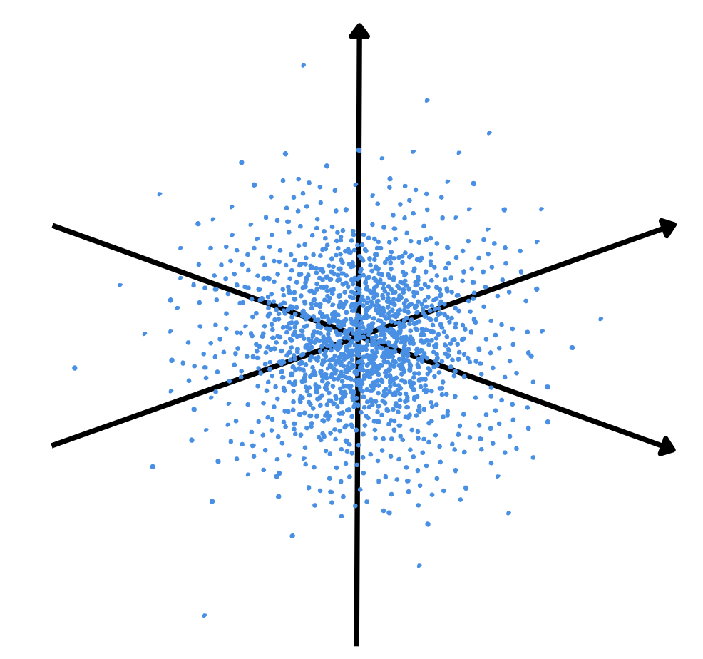
The central object is the wave function \( \Psi(x,t) \). It is not a material wave. It is a calculator for chances. The squared size gives a probability density for position and must integrate to one: \[ P(x,t)=|\Psi(x,t)|^2, \qquad \int_{-\infty}^{\infty} |\Psi(x,t)|^2\,dx=1. \] Normalization sets the overall scale of \( \Psi \). If you forget to normalize, you can still get pretty pictures but any number you read off will drift. In practice we often guess a shape for \( \Psi \), compute the integral of the square, and then divide by the square root of that integral so that the total area is one. This simple step is why many quantum calculations start with an integral before any physics appears.

Interference is already present in this viewpoint. If you add two allowed states, the probability is not just the sum of the two probabilities. It contains a cross term that depends on the relative phase. That one extra term explains the bright and dark bands in the double slit and many contrast effects in optics and matter wave experiments. You can see the role of phase without memorizing a new law. It is just a property of squaring a sum of complex numbers. Once you accept that amplitudes add and probabilities come from squares, most beginner paradoxes calm down quickly.

The time rule is the Schrödinger equation \[ i\hbar \frac{\partial}{\partial t}\Psi(x,t)=\hat{H}\,\Psi(x,t). \] The Hamiltonian \( \hat{H} \) is the energy operator. In most one dimensional examples \( \hat{H}= -\frac{\hbar^2}{2m}\frac{d^2}{dx^2}+V(x) \), which reads as kinetic energy plus potential energy. If the potential is steady in time, try a separable form \(\Psi(x,t)=\phi(x)\,e^{-iEt/\hbar}\). This turns the partial differential equation into a stationary one for \( \phi(x) \). You have seen this move in classical waves when you search for standing modes on a string. The same idea works here and it immediately suggests how boundaries control allowed shapes and energy levels.

You can learn a lot before solving exactly. If a wall forces \( \phi(x) \) to vanish at an edge, nodes must appear there. If the region is wider, more half waves can fit, which lowers the spacing between allowed energies. If the mass is larger, the kinetic term is harder to excite and levels decrease. These are limit checks that you can do in seconds. When your final expression agrees with them, your confidence rises for the right reasons. When it disagrees, you have a map for where to look. This is what it means to let physical reasoning steer the algebra instead of the other way around.

Superposition says that if \( \Psi_1 \) and \( \Psi_2 \) solve the same linear equation, then any combination \( c_1\Psi_1+c_2\Psi_2 \) also solves it. This is not an exotic quantum clause. It is a property of linear systems that you already used in simple harmonic motion and in wave addition on strings. What is new is the role of complex phase. The relative phase between pieces determines how they interfere later. If two paths are kept clean so that nothing records which way the particle went, their amplitudes add and a cross term appears after squaring. If a reliable record is made, the cross term fades and the pattern softens. The math is small. The effect is large.

A useful practice problem is to split a wave, delay one arm slightly, and recombine. Write the two pieces as \( \Psi_1=\Psi_0 \) and \( \Psi_2=\Psi_0 e^{i\phi} \). The combined probability is \( |\Psi_1+\Psi_2|^2=2|\Psi_0|^2(1+\cos\phi) \). The cosine term is the cross term and it is the whole story of fringe contrast. Anything in your setup that changes the phase difference shifts fringes. Anything that lets the environment learn which path was taken reduces the amplitude of the cosine term. This simple model is enough to understand many laboratory knobs without reading a long manual first.

The position spread \( \Delta x \) and momentum spread \( \Delta p \) obey \[ \Delta x\,\Delta p \ge \frac{\hbar}{2}. \] This is not about poor tools. It is built into the structure of wave functions and Fourier transforms. Squeezing a packet in space demands a wider range of momenta to build the sharp edges. That wider range makes the packet spread faster as it evolves in time. Designers use this fact as a knob. If you need stability in position for longer, you prepare a colder state with smaller momentum spread. If you need sharp spatial features for a short time, you accept rapid spreading and plan measurements accordingly. Thinking this way turns a limitation into a control strategy.

Classical motion stops at a wall when energy is too low. Quantum motion allows a small chance to appear beyond a thin or moderate barrier. Inside the barrier the amplitude decays exponentially but does not drop to zero instantly. At the far side a faint tail emerges. This view already explains scanning tunneling microscopes which measure currents from electrons tunneling through vacuum gaps only a nanometer wide. The same picture describes diodes that rely on controlled tunneling and nuclear alpha decay where a particle leaves the nucleus by leaking through a strong potential wall. You do not need the full derivation to remember safe trends: thicker barriers and heavier particles suppress the chance; lower barriers and lighter particles enhance it.

Spin is an intrinsic two state structure that behaves like a vector of operators. A simple model uses the basis \( |{\uparrow}_z\rangle \) and \( |{\downarrow}_z\rangle \) with a general state \( |\psi\rangle=\alpha |{\uparrow}_z\rangle+\beta |{\downarrow}_z\rangle \) where \( |\alpha|^2+|\beta|^2=1 \). A Stern Gerlach chain shows three reusable rules. Outcomes can be discrete even when the incoming beam looks smooth. Measuring along a new axis scrambles certainty built along the old axis. Repeating the same axis restores the earlier predictability. With only these lines you can already track simple qubit protocols and reason about rotations on the Bloch sphere without long matrices.

The average outcome of many runs is \[ \langle A \rangle = \int \Psi^*(x,t)\,\hat{A}\,\Psi(x,t)\,dx = \langle \psi | \hat{A} | \psi \rangle. \] This is a bookkeeping tool that unifies pictures. The integral form is perfect when you have functions of \(x\). The bra ket form is perfect when you manipulate finite bases like spin. In both cases your first check is units. If the operator reports a length, the final expression must carry length. Your second check is symmetry. If a transformation that should not change the physics flips the sign of your result, something in the setup needs attention. These two checks are fast and save hours later.

Some states are not products of parts. A compact example is the two qubit state \[ \frac{1}{\sqrt{2}}\big(|00\rangle + |11\rangle\big). \] No pair \( |a\rangle\otimes|b\rangle \) reproduces its perfect correlations. This does not send signals faster than light. It reflects how the state was prepared and how questions are asked. The safe habit is to treat the combined system first, then describe a part by tracing over what you ignore. That move sounds abstract but it is a simple average over the degrees of freedom you do not read out. With that you can predict what each lab arm will see without inventing extra forces or hidden variables.

A sharp projective measurement aligns outcomes with eigenvectors of an operator. Real experiments couple to surroundings. When the environment keeps a reliable record of which path was taken, the off diagonal terms of the reduced description shrink and the interference contrast falls. You did not break a conservation law. You changed the condition needed for phases to add. The practical lesson is short. If you want high contrast fringes, isolate the system and work quickly. If you want which path information, accept that contrast will drop. Knowing which knob does what turns confusion into planning.

The same small kit drives devices you meet in class and in labs. Band structure is a standing wave story in a periodic crystal and explains why semiconductors conduct only when you place electrons in certain ranges of energy. Lasers rely on controlled emission between energy levels and a resonator that feeds back the right phase so that light builds up rather than cancels. MRI manipulates spin with radio frequency pulses and gradient fields so that location tags appear in the frequency of the returning signal. Quantum sensors squeeze uncertainty to trade noise in one quantity for better resolution in another. You can tell a simple version of each device using only amplitude, phase, operators, and the checks you now use by habit.

Normalize a Gaussian and compute its width, then use the free packet spread formula to predict how long it takes that width to double for an electron and for a sodium atom. Sketch the first three standing waves in a box and explain node locations from the boundary conditions and from the idea of half waves that must fit exactly. Estimate how tunneling chance changes when the barrier thickness doubles while mass and kinetic energy stay fixed, and write a two line explanation of the trend in plain language. Model a Stern Gerlach chain with the middle magnet rotated by an angle and predict relative intensities at the three outputs using only superposition ideas. Compute one expectation value in integral form and in bra ket form and confirm the numbers match to build comfort switching between pictures.