Orientation
A toolkit is not a list to memorize. It is a way of thinking that lets you move from a question to a prediction without panic. In classical topics you may rely on forces, free body diagrams, and familiar algebra. In quantum work the objects change, but the spirit is the same. You learn what a state is, what an operator does, how probabilities appear, and how time evolution carries a system forward. Each piece looks abstract at first. With practice you will see the same shapes appear in different problems. That repetition is the point. You are training your eye to notice structure and your hand to write simple statements that a lab can check. As you read, do not hurry. Let each paragraph settle. Say it back in your own words, then store the line that makes sense to you in the notebook so you can return to it later and see how your understanding has shifted.
This page moves slowly on purpose. We will not sprint through every famous topic. We will build a few strong tools and use them. When a sentence feels heavy, say it back in your own words and save that version in the notebook. The goal is not to win a debate. The goal is to be clear, to learn to predict without mystery, and to separate what the math is telling you from what a picture in your head might suggest. If you treat each section as a short lab where you test one idea, the later chapters will feel familiar, and the jargon will feel like names for things you already know rather than a wall you have to climb.
The wavefunction
The central object of nonrelativistic quantum theory is the wavefunction, written with the symbol psi. It tells you how probability is distributed in space and time for a system. It is not a little cloud of matter. It is a complex valued function that carries amplitude and phase. You do not look at it directly. You use it to compute the chance of outcomes. If that sounds abstract, think of a recipe card. The card is not the cake but it tells you how to get the cake. In the same way the wavefunction is not the particle but it tells you how to predict what a careful apparatus will record. The shape of psi contains patterns like peaks and nodes that hint at where outcomes are likely and where they are rare, and those shapes depend on the physical situation you are describing.
Different systems use different variables. For a single particle in one dimension you write psi of x and t. For two particles you may write psi of x one and x two and t. For a spin system there may be no position at all in the description. None of that changes the basic role of the wavefunction. It is a compact way to encode what outcomes are possible and how likely they are when you perform a measurement that matches the description you chose. When you normalize psi so that the total probability is one, you are making sure your story about the system is consistent with the language of data. Later you can compute simple averages, like the average position or average energy, and you will see that the averages line up with what many repeated measurements would show in a real lab when the preparation is the same each time.
Probability from amplitudes
The probability rule turns the wavefunction into numbers a lab can check. Take the magnitude squared of psi and you get a probability density. That density tells you how likely it is to find the system with a position inside a small region. Integrate the density across the whole space and you should get one. That is the normalization condition. If you change the scale of psi so that this condition holds, your predictions will be consistent. This rule is simple to state and easy to forget under pressure, so write it in the margin whenever you start a problem. When you hear people talk about the Born rule, this is what they mean, a clean bridge from the abstract function to the frequencies of outcomes you would record if you ran the same experiment many times.
Worked example — normalization snapshot
Suppose ψ(x) is proportional to an exponential that decays with distance from the origin. Write a constant in front, square the magnitude, and integrate to fix the constant so that the total probability is one. The exact integral is a line or two with a standard table. The lesson is that normalization forces your function to speak the same probability language as the detector. It is a unit check for chance. Once normalized, you can also compute the average position which will sit at the center of the distribution, and the spread which tells you how wide the likely region is. These two numbers already give a useful picture before any heavy algebra appears.
Operators and observables
An observable is a physical quantity you can measure. In quantum theory each observable is represented by an operator that acts on the wavefunction. The operator is a rule. You feed ψ into it and it returns a new function. When that new function is simply a number times the original ψ, the state is called an eigenstate and the number is the eigenvalue that the measurement will return with certainty. Most states are not eigenstates of the quantity you care about. That is why probabilities appear. The operator language looks formal at first, but it is just a machine that connects your mathematical description to what a device can read. Common operators include the position operator, the momentum operator which looks like a derivative, and the Hamiltonian which gathers energy and interaction information into one object.
The expectation value is the average result of many identical trials. If you repeat the same preparation of the system and measure the same observable each time, the average result will approach this number. It is not a guess. It is a direct translation of the wavefunction and the operator into a prediction for data taken honestly. The best habit is to compute the expectation and also compute the spread so you know how sharp the prediction is. You will also hear about commutators, which measure whether the order of two operations matters. When two operators do not commute, you should expect a limit on how sharp both quantities can be at the same time, which is a practical warning about what any experiment can do.

Time evolution and the Schrödinger rule
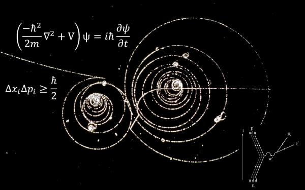
A state does not sit still unless the system is arranged that way. The Schrödinger equation tells you how ψ changes with time. It plays the role that Newton’s second law plays in mechanics. Give the Hamiltonian which encodes energy and interactions and the rule carries the state forward. The equation looks short. Its content is deep. Solving it is how you get from a preparation at time zero to a prediction for an outcome at a later time. When the Hamiltonian does not depend on time, the story is cleaner. When it does, you still have a recipe to follow step by step. Boundary conditions matter as much as the rule itself, since they pick which patterns are allowed in the first place.
Worked example — stationary states in a simple well
A particle in a one dimensional box has solutions that are standing waves. Each allowed shape comes with a specific energy. If the system is prepared in one of these shapes, the probability density does not change in time even though the wavefunction itself picks up a time dependent phase. This is the simplest case where the mathematics separates into a space part that sets patterns and a time part that keeps the rhythm. The same separation appears in many textbook problems and it is a useful habit to look for it before trying anything more complicated because it turns a large puzzle into two smaller ones you can solve cleanly.

Superposition and interference
If two states are possible, the sum is also a state. That simple linear rule is called superposition. It is not a metaphor. It is the reason interference patterns appear. Add two amplitudes and then square the magnitude to get probabilities and you will see cross terms that can help or cancel. When paths remain undisturbed those cross terms survive and produce bright and dark regions on a screen. When a reliable record of which path was taken exists, the cross terms are suppressed and the pattern becomes a simple sum. Learning to predict when interference survives is a core skill in this subject. Coherence is the word you will hear for the quiet alignment that keeps phases in step so that interference can show itself.
Worked example — two path phase shift
Two paths deliver amplitudes with the same size to a point on a screen. If the relative phase is zero, the probability at that point is large. If the relative phase is one hundred and eighty degrees, the probability is small. A small change in path length or refractive index can move a bright region to a dark region. This is the simplest laboratory handle you will use again and again in optics and in other wave systems. The same story appears with sound in a room or ripples on a pond, which is a nice reminder that quantum is strange in its rules but familiar in many of its patterns.
Measurement and update
Before a measurement a state can be a superposition of outcomes. After a sharp measurement you record one result. The way we connect those statements is to update the state according to the outcome observed. There is debate about whether this update represents something happening in the world or a change in our information. You do not need to settle that debate to solve problems. What matters is that your predictions for sequences of measurements match what a good experiment will produce. The update rule is the practical bridge between preparation, action, and record. If you measure the same quantity right away again in a well controlled setup, you should get the same result, which is a helpful check that your description matches what the apparatus is doing.
Spin as a two state system
Spin does not mean a tiny sphere is literally turning. It is an intrinsic two state property that behaves like an arrow you can test along different directions. If you prepare spin up along a vertical axis and then test along the same axis you will get up with certainty. If you test along a horizontal axis you will see up half the time and down half the time. The language of two state systems is a perfect place to practice superposition and measurement without the extra detail of position. Many modern technologies use spin like a bit that can also point between the basic directions during a calculation. The simple picture of filters that pass only one orientation is enough to build a mental model you can trust while you learn the formal steps.
Entanglement in plain words
Two systems can share a state that cannot be written as a simple product of two separate states. That is entanglement. It means that the best description of the parts requires the whole. When you measure one system the results you get are correlated with results on the other in ways that no simple shared list of hidden properties can explain. This is not science fiction. It is a pattern confirmed in careful tests. For our purposes it is a tool. Entanglement lets information be shared and processed in ways that would be impossible with independent parts. It is also a reminder to be careful about assuming that systems have their own stories when the mathematics is telling you otherwise. At the level of a toolkit, remember only that correlations can be stronger than any classical picture would allow and that those correlations are useful when designed with care.
Decoherence and why everyday life looks classical
Quantum interference relies on delicate phase relations between parts of a state. Interaction with a complex environment tends to spread that phase information into many degrees of freedom. When that happens the cross terms that gave interference are practically lost and predictions reduce to simple sums. The system has not changed its fundamental rules. We have lost access to the information needed to see the quantum pattern. This process is called decoherence. It explains why tables and planets look classical even if the building blocks obey quantum rules. For the working student the lesson is that isolation and control are real resources in any quantum experiment. Shielding, cooling, and short times between preparation and measurement are not luxuries, they are the basic tools that keep coherence alive long enough to study.
Putting the tools to work
A typical problem starts with a preparation statement. You choose an initial wavefunction or a spin direction. You normalize it so the total probability is one. You identify the observable of interest and write the operator. You use the Schrödinger rule to evolve the state if time passes before the measurement. You compute the expectation or the distribution of outcomes. Then you check limits where the answer should be simple. If you have two different paths to the same number and they agree you have strong evidence that the calculation is sound. This workflow is not exciting to read about but it is powerful to use. It keeps your work honest and repeatable. When you write your final sentence, say what would happen if a key parameter doubled or if it were cut in half, since that gives the result a shape a reader can remember and test.
Practice prompts
Try these as one page exercises. One. Write a simple gaussian wavefunction and normalize it. Two. For that state compute the expectation of position and the spread and explain what those numbers tell you about where the particle is likely to be found. Three. Consider a two path setup where the paths have equal amplitude but a controllable phase. Predict the probability at a chosen point as the phase is adjusted. Four. Prepare a spin up state along a vertical axis and compute the probabilities for tests along a horizontal axis. Five. Explain in your own words how decoherence changes interference patterns without breaking basic rules. Six. Sketch a potential well of your choice and describe qualitatively what the lowest two stationary states might look like before you do any algebra at all.
Toolkit quiz
1) What does |ψ(x)|² represent
2) An eigenstate of an operator has which property
3) The Schrödinger equation tells you
4) Interference fades when
5) The expectation value ⟨A⟩ is
6) Superposition means
7) Decoherence explains
8) A spin prepared up along z and then measured along x gives
9) The main role of an operator in this toolkit is
10) Normalization ensures
Glossary
Amplitude: the complex number carried by the wavefunction at a point. The square of its magnitude gives probability density. Phase is the angle of that number and is what allows interference to build or cancel. Normalization: the condition that total probability equals one, which fixes any overall scale factor in the wavefunction. Operator: a rule that acts on states and represents an observable like position, momentum, or energy. Hermitian operators are the ones whose outcomes are real numbers which is why they represent measurable things.
Eigenstate and eigenvalue: special cases where the action of an operator returns the same state times a number, which means a sharp measurement result. Hamiltonian: the operator that gathers energy terms and generates time evolution through the Schrödinger equation. Superposition: the rule that sums of allowed states are also allowed states which leads directly to interference patterns. Decoherence: the practical loss of phase information to the environment that makes predictions look classical at large scales even though the rules remain quantum underneath.